Gaussian Elimination

Row Eschelon Form :drill:

A matrix is said to be in [row-eschelon form] if it satisfies the following conditions:

1. All zero rows (consisting only of zeros) are [at the bottom].
2. Each leading entry is to the [right] of all leading entreis in the row above it.
3. All entries below a leading entry are [zero].

Broken examples $\left[\begin{array}{ccc}1& 0& 3\\ 0& 2& 1\\ 0& 0& 0\end{array}\right]$

Invalid b/c it violates rule 2 above in row 2.

$\left[\begin{array}{ccc}1& 0& 3\\ 0& 1& 2\\ 0& 1& 0\end{array}\right]$

Violates rule 3 above in row 3.

$\left[\begin{array}{ccc}1& 0& 3\\ 0& 0& 0\\ 0& 0& 0\end{array}\right]$

Violates rule 1 in row 2.

Good examples $\left[\begin{array}{ccc}1& \ast & \ast \\ 0& 0& 1\end{array}\right]$

$\left[\begin{array}{cccc}0& 1& \ast & \ast \\ 0& 0& 1& \ast \\ 0& 0& 0& 0\end{array}\right]$

$\left[\begin{array}{ccc}1& \ast & \ast \\ 0& 1& \ast \\ 0& 0& 1\end{array}\right]$

$\left[\begin{array}{cccc}0& 1& \ast & \ast \\ 0& 0& 1& \ast \\ 0& 0& 0& 0\end{array}\right]$

$\left[\begin{array}{cccc}1& \ast & \ast & 0\\ 0& 1& \ast & 0\\ 0& 0& 0& 1\end{array}\right]$

Reduced row-eschelon form :drill: Scheduled: 2022-10-28 A row-eschelon matrix is said to be in [reduced row-eschelon form] if in addition it satisfies the following condition:

1. Must be in [Row Eschelon Form]
2. [Each leading 1 is the only nonzero entry in it’s column]
3. [The first non-zero entry from the left in each non-zero row is a 1]. This is called [a leading one] for that row.

Good examples $\left[\begin{array}{ccc}1& \ast & 0\\ 0& 0& 1\end{array}\right]$

$\left[\begin{array}{cccc}0& 1& 0& \ast \\ 0& 0& 1& \ast \\ 0& 0& 0& 0\end{array}\right]$

$\left[\begin{array}{cccc}1& 0& \ast & 0\\ 0& 1& \ast & 0\\ 0& 0& 0& 0\end{array}\right]$

$\left[\begin{array}{ccc}1& 0& 0\\ 0& 1& 0\\ 0& 0& 1\end{array}\right]$

Pivots :drill: Once a matrix is in Reduced row-eschelon form, the leading 1’s are called [pivots] and the column that contains them are called [pivot columns].

Theorem 1.2.1 :drill: Scheduled: 2022-10-28 Theorem: Every matrix can be brought to (reduced) row-eschelon form by a sequence of [elementary row operations].

Gaussian Algorithm :math:drill:

Scheduled: 2022-10-22

1. If a matrix is a zero matrix, [there’s nothing to do].
2. Otherwise, find the first column from the [left] containing a non-zero entry (called a) and move the row containing it to the top position.
3. multiply the first row by [the reciprocal] of the non-zero to get 1.
4. By [subtracting multiples|operation] of that row from rows below it, make each entry the leading 1 zero (this completes the first row)
5. Repeat steps 1-4 on the matrix for the remaining rows. the process stops when either [no rows remain] or [the remaining rows are zero]

Example $\left[\begin{array}{cc}0& 0\\ 0& \ast \\ 0& \ast \end{array}\right]$

$\left[\begin{array}{cc}0& \ast \\ 0& 0\\ 0& \ast \end{array}\right]$

$\left[\begin{array}{cc}0& 1/\ast \\ 0& 0\\ 0& \ast \end{array}\right]$

$\left[\begin{array}{cc}0& 1\\ 0& 0\\ 0& \ast \end{array}\right]$

Solve the following $\{\begin{array}{l}3x-4z=-1\\ x+10z=5\\ 4x+y+6z=1\end{array}$

Augmented matrix is: $\left[\begin{array}{ccc}3& 1& -4|-1\\ 1& 0& 10|5\\ 4& 1& 6|1\end{array}\right]$

r1←>r2 $\left[\begin{array}{ccc}1& 0& 10|5\\ 3& 1& -4|-1\\ 4& 1& 6|1\end{array}\right]$

r2: r2-r1*3 $\left[\begin{array}{ccc}1& 0& 10|5\\ 0& 1& -34|-16\\ 4& 1& 6|1\end{array}\right]$

r3: r3-r1*4 $\left[\begin{array}{ccc}1& 0& 10|5\\ 0& 1& -34|-16\\ 0& 1& -34|-19\end{array}\right]$

r3: r3-r2 $\left[\begin{array}{ccc}1& 0& 10|5\\ 0& 1& -34|-16\\ 0& 0& 0|-3\end{array}\right]$ (this is reduced row-eschelon form)

Final system turns into $\{\begin{array}{l}x+10z=5\\ y-34z=-16\\ 0=-3\end{array}$

It’s equivalent b/c we only used Elementary row operation rules. It’s inconsistent b/c $0\ne -3$. hence there is no solution.

Solve the following

$\{\begin{array}{l}{x}_1-2x_2-x_3+3x_4=1\\ 2x_1-4x_2+x_3=5\\ x_1-2x_2+2x_3-3x_4=4\end{array}$

$\left[\begin{array}{cccc}1& -2& -1& 3|1\\ 2& -4& 1& 0|5\\ 1& -2& 2& -3|4\end{array}\right]$

r2:r2-2*r1 $\left[\begin{array}{cccc}1& -2& -1& 3|1\\ 0& 0& 3& -6|3\\ 1& -2& 2& -3|4\end{array}\right]$

r3: r3-r1 $\left[\begin{array}{cccc}1& -2& -1& 3|1\\ 0& 0& 3& -6|3\\ 0& 0& 3& -6|3\end{array}\right]$

r2: 1/3 \ast r2 $\left[\begin{array}{cccc}1& -2& -1& 3|1\\ 0& 0& 1& -2|1\\ 0& 0& 3& -6|3\end{array}\right]$

r3: r3-3*r2 $\left[\begin{array}{cccc}1& -2& -1& 3|1\\ 0& 0& 1& -2|1\\ 0& 0& 0& 0|0\end{array}\right]$ — get to reduced form

r1=r1+r2 $\left[\begin{array}{cccc}1& -2& 0& 1|2\\ 0& 0& 1& -2|1\\ 0& 0& 0& 0|0\end{array}\right]$

Leading variables

The leading variables are the columns which have a leading 1. The non-leading variables are assigned parameters, so set x_2=s, x_4=t where s and t are arbitrary numbers. Then we solve it in terms of the leading variables.

We will always have an infinite number of solutions if the number of leading 1s are less than the number of columns.

Gaussian Elimination solution process :drill:

Scheduled: 2022-10-22 To solve a Systems of Linear Equations, proceed as follows:

1. Carry the augmennted matrix to a [reduced row-eschelon form].
2. If the matrix is of the form $\left[\begin{array}{ccc}0& 0& 0|\ast \end{array}\right]$

..[there is no solution].

3. Otherwise, assign the nonleading variables (if any) as parameters (e.g. s & t) and use the equation to solve for the leading variables in terms of the parameters.

Rank :drill: The [rank] is the count of leading ones in any row-eschelon matrix. Rank (r) is ⇐ m and r ⇐ n in an $m\cdot n$ matrix.

Example $A=\left[\begin{array}{cccc}1& 1& -1& 4\\ 2& 1& 3& 0\\ 0& 1& -5& 8\end{array}\right]$

r2 = r2 - 2*r1 $\left[\begin{array}{cccc}1& 1& -1& 4\\ 0& -1& 5& -8\\ 0& 1& -5& 8\end{array}\right]$

r2 ←> r3 $\left[\begin{array}{cccc}1& 1& -1& 4\\ 0& 1& -5& 8\\ 0& -1& 5& -8\end{array}\right]$

r3 = r3 + r2 $\left[\begin{array}{cccc}1& 1& -1& 4\\ 0& 1& -5& 8\\ 0& 0& 0& 0\end{array}\right]$

— reduce it r1 = r1 - r2 $\left[\begin{array}{cccc}1& 0& 4& -4\\ 0& 1& -5& 8\\ 0& 0& 0& 0\end{array}\right]$

— Because the row eschelon matix has 2 leading ones, it’s rank of the original matrix $A$ is 2.

Theorem 1.2.2 :drill: Suppose a system of m equations in n variables is consistent and that the rank is of the augmented matrix is r.

1. The set of solutions involves exactly n-r parameters. (e.g. n-r = [the count of non-leading variables|what does this describe])
2. if r=n, the system has [a unique solution|what sort of solution].
3. if r < n, the system has [infinitely many solutions|what sort of solution].

For any system of linear equations, exactly 3 possibilities exist.

1. no solution: this occurs when a row like $\left[\begin{array}{cccc}0& 0& ...& 0|\ast \end{array}\right]$ occurs in the row eschelon form.
2. unique solution: Every variable is a leading variable.
3. infinitely many solutions: There are non-leading variables.

Homework 1.2

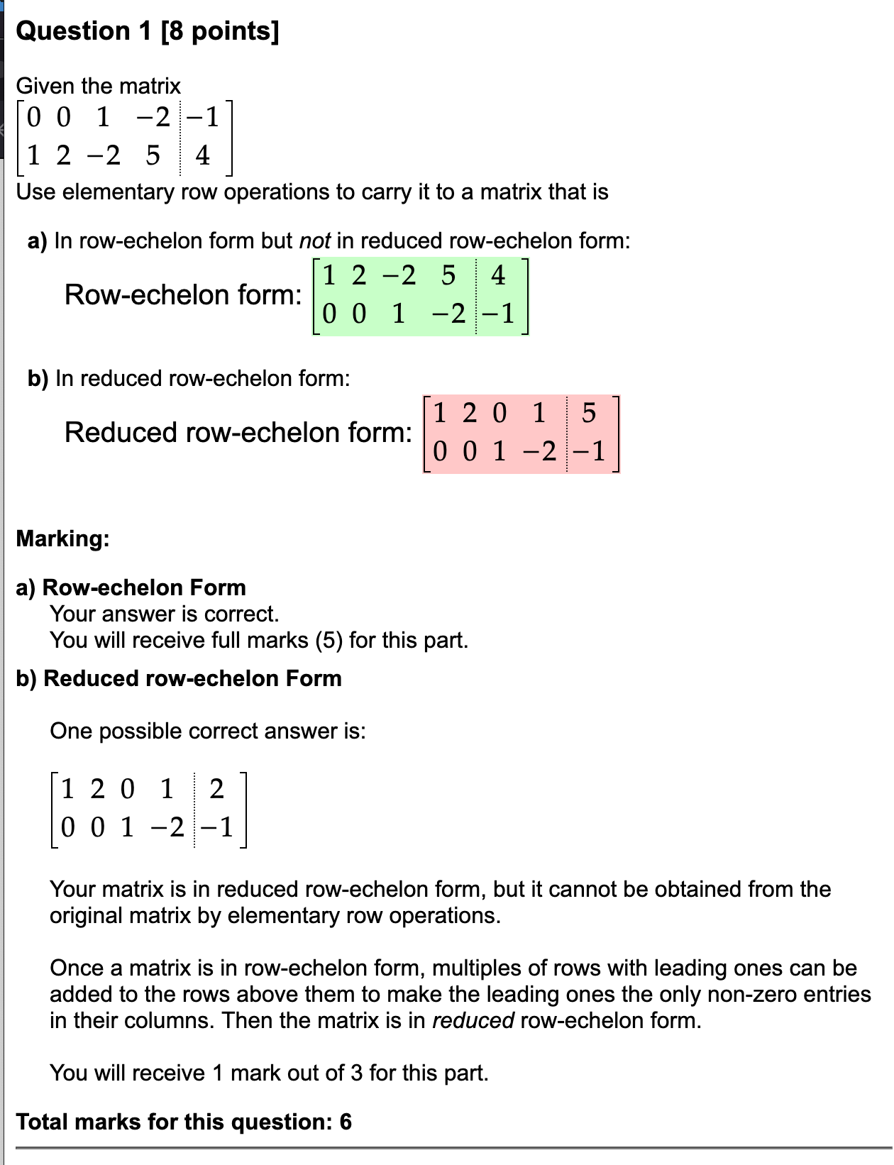
q1

Use elementary row operations to carry it to a matrix that is

In row-echelon form but not in reduced row-echelon form:

$\left[\begin{array}{cccccc}0& 0& 1& -2& |& -1\\ 1& 2& -2& 5& |& 4\end{array}\right]$

r1←>r2 $\left[\begin{array}{cccccc}1& 2& -2& 5& |& 4\\ 0& 0& 1& -2& |& -1\end{array}\right]$

In reduced row-echelon form: r1 = r1+2*r2 $\left[\begin{array}{cccccc}1& 2& 0& 1& |& 3\\ 0& 0& 1& -2& |& -1\end{array}\right]$

—

Got it wrong b/c I did -1^2 not -1*2. That said, the correct answer theyu say is 2 in the top right, which doesn’t make sense to me.

q1-2 $\left[\begin{array}{cccccc}2& -4& 2& 2& |& -2\\ 1& -2& 1& 2& |& 2\end{array}\right]$

row eschelon form r1=r1-2*r2 $\left[\begin{array}{cccccc}0& 0& 0& -2& |& -6\\ 1& -2& 1& 2& |& 2\end{array}\right]$

r1←>r2 $\left[\begin{array}{cccccc}1& -2& 1& 2& |& 2\\ 0& 0& 0& -2& |& -6\end{array}\right]$

r2 = -1/2 \ast r2 $\left[\begin{array}{cccccc}1& -2& 1& 2& |& 2\\ 0& 0& 0& 1& |& 3\end{array}\right]$

reduced row-eschelon r1 = r1-2*r2 $\left[\begin{array}{cccccc}1& -2& 1& 0& |& -4\\ 0& 0& 0& 1& |& 3\end{array}\right]$

q2

Given the matrix, get it to reduced row-eschelon form $\left[\begin{array}{ccccccc}0& -3& -9& -6& -3& |& 12\\ 0& 2& 6& 4& 4& |& -8\\ 1& 3& 4& 6& -1& |& -11\end{array}\right]$

r1←>r3 $\left[\begin{array}{ccccccc}1& 3& 4& 6& -1& |& -11\\ 0& 2& 6& 4& 4& |& -8\\ 0& -3& -9& -6& -3& |& 12\end{array}\right]$

r3=r1+r3 $\left[\begin{array}{ccccccc}1& 3& 4& 6& -1& |& -11\\ 0& 2& 6& 4& 4& |& -8\\ 0& 0& -5& 0& -4& |& 1\end{array}\right]$

r2 = 1/2 \ast r2 $\left[\begin{array}{ccccccc}1& 3& 4& 6& -1& |& -11\\ 0& 1& 3& 2& 2& |& -4\\ 0& 0& -5& 0& -4& |& 1\end{array}\right]$

r1=r1-3*r2 $\left[\begin{array}{ccccccc}1& 0& -5& 0& -7& |& 1\\ 0& 1& 3& 2& 2& |& -4\\ 0& 0& -5& 0& -4& |& 1\end{array}\right]$

r3=-1/5 \ast r3 $\left[\begin{array}{ccccccc}1& 0& -5& 0& -7& |& 1\\ 0& 1& 3& 2& 2& |& -4\\ 0& 0& 1& 0& 4/5& |& -1/5\end{array}\right]$

r1=r1+5*r3 $\left[\begin{array}{ccccccc}1& 0& 0& 0& -3& |& 0\\ 0& 1& 3& 2& 2& |& -4\\ 0& 0& 1& 0& 4/5& |& -1/5\end{array}\right]$

r2=r2-3*r3 $\left[\begin{array}{ccccccc}1& 0& 0& 0& -3& |& 0\\ 0& 1& 0& 2& -2/5& |& -17/5\\ 0& 0& 1& 0& 4/5& |& -1/5\end{array}\right]$

— Got it wrong.

Your matrix is in reduced row-echelon form, but it cannot be obtained from the original matrix by elementary row operations.

The Gaussian Algorithm can be used to carry a matrix to row-echelon form. Once a matrix is in row-echelon form, multiples of rows with leading ones can be added to the rows above them to make the leading ones the only non-zero entries in their columns. Then the matrix is in reduced row-echelon form.

You will receive 1 mark out of 3 for this part.

Valid: $\left[\begin{array}{ccccccc}1& 0& -5& 0& 0& |& 1\\ 0& 1& 3& 2& 0& |& -4\\ 0& 0& 0& 0& 1& |& 0\end{array}\right]$

q2-2 $\left[\begin{array}{ccccccc}1& -3& 2& 2& 4& |& 9\\ 1& 0& -1& 2& -2& |& -3\\ 1& -1& 1& 2& 4& |& 4\end{array}\right]$

r2=r2-r1 $\left[\begin{array}{ccccccc}1& -3& 2& 2& 4& |& 9\\ 0& 3& -3& 0& -6& |& -12\\ 1& -1& 1& 2& 4& |& 4\end{array}\right]$

r3=r3-r1 $\left[\begin{array}{ccccccc}1& -3& 2& 2& 4& |& 9\\ 0& 3& -3& 0& -6& |& -12\\ 0& 2& -1& 0& 0& |& -5\end{array}\right]$

r2=r2*1/3 $\left[\begin{array}{ccccccc}1& -3& 2& 2& 4& |& 9\\ 0& 1& -1& 0& -2& |& -4\\ 0& 2& -1& 0& 0& |& -5\end{array}\right]$

r3=r3-2*r2 $\left[\begin{array}{ccccccc}1& -3& 2& 2& 4& |& 9\\ 0& 1& -1& 0& -2& |& -4\\ 0& 0& 1& 0& 2& |& 3\end{array}\right]$

now to get reduced REF r1=r1+3*r2 $\left[\begin{array}{ccccccc}1& 0& -1& 2& -2& |& -3\\ 0& 1& -1& 0& -2& |& -4\\ 0& 0& 1& 0& 2& |& 3\end{array}\right]$

r2=r2+r3 $\left[\begin{array}{ccccccc}1& 0& -1& 2& -2& |& -3\\ 0& 1& 0& 0& 0& |& -1\\ 0& 0& 1& 0& 2& |& 3\end{array}\right]$

r1=r1+r3 $\left[\begin{array}{ccccccc}1& 0& 0& 2& 0& |& 0\\ 0& 1& 0& 0& 0& |& -1\\ 0& 0& 1& 0& 2& |& 3\end{array}\right]$

— wrong Correct: $\left[\begin{array}{cccccc}1& 0& 0& 2& 2& |0\\ 0& 1& 0& 0& 2& |-1\\ 0& 0& 1& 0& 4& |-3\end{array}\right]$

q2-3 $\left[\begin{array}{ccccccc}0& 0& -1& -2& -1& |& 3\\ 0& 0& 5& 10& 10& |& -15\\ 1& 4& -1& -6& -1& |& 8\end{array}\right]$

r1←>r3 $\left[\begin{array}{ccccccc}1& 4& -1& -6& -1& |& 8\\ 0& 0& -1& -2& -1& |& 3\\ 0& 0& 5& 10& 10& |& -15\end{array}\right]$

r3=r3+5*r2 $\left[\begin{array}{ccccccc}1& 4& -1& -6& -1& |& 8\\ 0& 0& -1& -2& -1& |& 3\\ 0& 0& 0& 0& 5& |& 0\end{array}\right]$

r2=-1 \ast r2 $\left[\begin{array}{ccccccc}1& 4& -1& -6& -1& |& 8\\ 0& 0& 1& 2& 1& |& -3\\ 0& 0& 0& 0& 5& |& 0\end{array}\right]$

r3=1/5 \ast r3 $\left[\begin{array}{ccccccc}1& 4& -1& -6& -1& |& 8\\ 0& 0& 1& 2& 1& |& -3\\ 0& 0& 0& 0& 1& |& 0\end{array}\right]$

— now reduced REF

r1=r1+r2 $\left[\begin{array}{ccccccc}1& 4& 0& -4& 0& |& 5\\ 0& 0& 1& 2& 1& |& -3\\ 0& 0& 0& 0& 1& |& 0\end{array}\right]$

r2=r2-r3 $\left[\begin{array}{ccccccc}1& 4& 0& -4& 0& |& 5\\ 0& 0& 1& 2& 0& |& -3\\ 0& 0& 0& 0& 1& |& 0\end{array}\right]$

q3

The reduced row-echelon form of the augmented matrix for a system of linear equations with variables x1, … , x4 is given below. Determine the solutions for the system and enter them below.

$\left[\begin{array}{cccccc}1& 0& 4& -4& |& -2\\ 0& 1& 4& 1& |& -3\end{array}\right]$

$\begin{array}{rl}x1+4x3-4x4& =-2\\ x1+4s-4t& =-2\\ x1& =-4s+4t-2\end{array}$

$\begin{array}{rl}{x}_2+4s+t& =-3\\ x_2& =-4s-t-3\end{array}$

q4

The reduced row-echelon form of the augmented matrix for a system of linear equations with variables x1, … , x5 is given below. Determine the solutions for the system and enter them below.

$\left[\begin{array}{ccccccc}1& -2& 0& 0& 4& |& 0\\ 0& 0& 1& 0& 4& |& -3\\ 0& 0& 0& 1& 2& |& 3\end{array}\right]$

$\begin{array}{rl}{x}_1-2r+4t& =0\\ x_1& =2r-4t\\ x_3+4t& =-3\\ x_3=-4t-3& \\ x_4+2t& =3\\ x_4=-2t+3& \end{array}$

q5

Solve the following system $\{\begin{array}{l}{x}_1-x_2+2x_3=-1\\ 2x_1-2x_2+5x_3=0\end{array}$

$\left[\begin{array}{ccccc}1& -1& 2& |& -1\\ 2& -2& 5& |& 0\end{array}\right]$

r2=r2-2*r1 $\left[\begin{array}{ccccc}1& -1& 2& |& -1\\ 0& 0& 1& |& -2\end{array}\right]$

$\begin{array}{rl}{x}_1-r-2x_3& =-1\\ x_1& =r+2x_3-1\\ x_3=-2& \end{array}$ — wrong $\begin{array}{r}{x}_1=-5+r\\ x_2=r\\ x_3=2\end{array}$

q5-2 $\{\begin{array}{l}2x_1-4x_2-10x_3=-28\\ -x_1+3x_2+8x_3=19\end{array}$

$\left[\begin{array}{ccccc}2& -4& -10& |& -28\\ -1& 3& 8& |& 19\end{array}\right]$

r1=1/2 \ast r1 $\left[\begin{array}{ccccc}1& -2& -5& |& -14\\ -1& 3& 8& |& 19\end{array}\right]$

r2=r1+r2 $\left[\begin{array}{ccccc}1& -2& -5& |& -14\\ 0& 1& 3& |& 5\end{array}\right]$

r1=r1+2*r2 $\left[\begin{array}{ccccc}1& 0& 1& |& -4\\ 0& 1& 3& |& 5\end{array}\right]$

$\begin{array}{rl}{x}_1+r& =-4\\ x_1& =-4-r\\ x_2+3r& =5\\ x_2& =5-3r\end{array}$

r6

Solve the following system of linear equations:

$\{\begin{array}{ll}4x_2-8x_3& =-10\\ 2x_2-4x_3& =-6\\ x_1+2x_2-3x_3& =-1\end{array}$

If the system has no solution, demonstrate this by giving a row-echelon form of the augmented matrix for the system.

$\left[\begin{array}{ccccc}0& 4& 8& |& -10\\ 0& 2& -4& |& -6\\ 1& 2& -3& |& -1\end{array}\right]$

r3←>r1 $\left[\begin{array}{ccccc}1& 2& -3& |& -1\\ 0& 4& 8& |& -10\\ 0& 2& -4& |& -6\end{array}\right]$

r2←>r3 $\left[\begin{array}{ccccc}1& 2& -3& |& -1\\ 0& 2& -4& |& -6\\ 0& 4& 8& |& -10\end{array}\right]$

r2=r2*1/2 $\left[\begin{array}{ccccc}1& 2& -3& |& -1\\ 0& 1& -2& |& -3\\ 0& 4& 8& |& -10\end{array}\right]$

r1=r1-2*r2 $\left[\begin{array}{ccccc}1& 0& 3& |& 5\\ 0& 1& -2& |& -3\\ 0& 4& 8& |& -10\end{array}\right]$

r3=r3-r2*4 $\left[\begin{array}{ccccc}1& 0& 3& |& 5\\ 0& 1& -2& |& -3\\ 0& 0& 16& |& 2\end{array}\right]$

r3=r3*1/16 $\left[\begin{array}{ccccc}1& 0& 3& |& 5\\ 0& 1& -2& |& -3\\ 0& 0& 1& |& 2/16\end{array}\right]$

r2=r2+2*r3 $\left[\begin{array}{ccccc}1& 0& 3& |& 5\\ 0& 1& 0& |& -11/4\\ 0& 0& 1& |& 2/16\end{array}\right]$

r1=r1-3*r3 $\left[\begin{array}{ccccc}1& 0& 0& |& 17/4\\ 0& 1& 0& |& -11/4\\ 0& 0& 1& |& 2/16\end{array}\right]$ — wrong

no solutions REF matrix: $\left[\begin{array}{ccccc}1& 2& -3& |& -1\\ 0& 1& -2& |& -3\\ 0& 0& 0& |& 1\end{array}\right]$

r6-2 $\{\begin{array}{l}5x_1-10x_2-10x_3=15\\ -x_1+5x_2+8x_3=0\\ 2x_1-2x_2=9\end{array}$

$\left[\begin{array}{ccccc}5& -10& -10& |& 15\\ -1& 5& 8& |& 0\\ 2& -2& 0& |& 9\end{array}\right]$

r1=r1*1/5 $\left[\begin{array}{ccccc}1& -2& -2& |& 3\\ -1& 5& 8& |& 0\\ 2& -2& 0& |& 9\end{array}\right]$

r2=r2+r1 $\left[\begin{array}{ccccc}1& -2& -2& |& 3\\ 0& 3& 6& |& 3\\ 2& -2& 0& |& 9\end{array}\right]$

r3=r3-2*r1 $\left[\begin{array}{ccccc}1& -2& -2& |& 3\\ 0& 3& 6& |& 3\\ 0& 2& 4& |& 3\end{array}\right]$

r2=r2/3 $\left[\begin{array}{ccccc}1& -2& -2& |& 3\\ 0& 1& 2& |& 1\\ 0& 2& 4& |& 3\end{array}\right]$

r3=r3-2*r2 $\left[\begin{array}{ccccc}1& -2& -2& |& 3\\ 0& 1& 2& |& 1\\ 0& 0& 0& |& 1\end{array}\right]$

r7 $\{\begin{array}{l}5x_1-5x_2-10x_3=15\\ 3x_1-3x_3=12\\ 2x_1-x_3=8\end{array}$

$\left[\begin{array}{ccccc}5& -5& -10& |& 15\\ 3& 0& -3& |& 12\\ 2& 0& -1& |& 8\end{array}\right]$

r1=r1/5 $\left[\begin{array}{ccccc}1& -1& -2& |& 3\\ 3& 0& -3& |& 12\\ 2& 0& -1& |& 8\end{array}\right]$

r2=r2-3*r1 $\left[\begin{array}{ccccc}1& -1& -2& |& 3\\ 0& -3& 3& |& 3\\ 2& 0& -1& |& 8\end{array}\right]$

r3=r3-2*r1 $\left[\begin{array}{ccccc}1& -1& -2& |& 3\\ 0& -3& 3& |& 3\\ 0& 2& 3& |& 2\end{array}\right]$

r2←>r3 $\left[\begin{array}{ccccc}1& -1& -2& |& 3\\ 0& 2& 3& |& 2\\ 0& -3& 3& |& 3\end{array}\right]$

r2=r2/2 $\left[\begin{array}{ccccc}1& -1& -2& |& 3\\ 0& 1& 3/2& |& 1\\ 0& -3& 3& |& 3\end{array}\right]$

r3=r3+r2*3 $\left[\begin{array}{ccccc}1& -1& -2& |& 3\\ 0& 1& 3/2& |& 1\\ 0& 0& 15/2& |& 6\end{array}\right]$

r3=r3/(15/2) $\left[\begin{array}{ccccc}1& -1& -2& |& 3\\ 0& 1& 3/2& |& 1\\ 0& 0& 1& |& 0.8\end{array}\right]$

$\begin{array}{rl}{x}_1-x_2-2x_3& =3\\ x_1& =x_2+2x_3+3\\ x_2+1.5x_3& =1\\ x_2& =-1.5x_3+1\\ x_3& =0.8\end{array}$ — wrong

correct: $\{\begin{array}{l}{x}_1=4\\ x_2=1\\ x_3=0\end{array}$

q7-2 (initial augmented matrix was wrong) $\{\begin{array}{l}{x}_1+x_2-x_3=-9\\ -3x_1+9x_3=6\\ -x_1+4x_3=1\end{array}$

$\left[\begin{array}{ccccc}1& 2& -1& |& -9\\ -3& 0& 9& |& 6\\ -1& 0& 4& |& 1\end{array}\right]$

r3=r1+r3 $\left[\begin{array}{ccccc}1& 2& -1& |& -9\\ -3& 0& 9& |& 6\\ 0& 2& 3& |& -8\end{array}\right]$

r2=r1*3+r2 $\left[\begin{array}{ccccc}1& 2& -1& |& -9\\ 0& 6& 6& |& -21\\ 0& 2& 3& |& -8\end{array}\right]$

r2=r2/6 $\left[\begin{array}{ccccc}1& 2& -1& |& -9\\ 0& 1& 1& |& -3.5\\ 0& 2& 3& |& -8\end{array}\right]$

r1=r1-2*r2 $\left[\begin{array}{ccccc}1& 0& -3& |& -2\\ 0& 1& 1& |& -3.5\\ 0& 2& 3& |& -8\end{array}\right]$

r3=r3-2*r2 $\left[\begin{array}{ccccc}1& 0& -3& |& -2\\ 0& 1& 1& |& -3.5\\ 0& 0& 1& |& -1\end{array}\right]$

r2=r2-r3 $\left[\begin{array}{ccccc}1& 0& -3& |& -2\\ 0& 1& 0& |& -2.5\\ 0& 0& 1& |& -1\end{array}\right]$

r1=r1+3*r3 $\left[\begin{array}{ccccc}1& 0& 0& |& -5\\ 0& 1& 0& |& -2.5\\ 0& 0& 1& |& -1\end{array}\right]$ —wrong correct: $\{\begin{array}{l}{x}_1=-5\\ x_2=-5\\ x_3=-1\end{array}$

q7-3 $\{\begin{array}{l}2x_2-4x_3=-2\\ x_1-3x_2+3x_3=1\\ -3x_2+7x_3=3\end{array}$

$\left[\begin{array}{ccccc}0& 2& -4& |& -2\\ 1& -3& 3& |& 1\\ 0& -3& 7& |& 3\end{array}\right]$

r1←>r2 $\left[\begin{array}{ccccc}1& -3& 3& |& 1\\ 0& 2& -4& |& -2\\ 0& -3& 7& |& 3\end{array}\right]$

r2 /= 2 $\left[\begin{array}{ccccc}1& -3& 3& |& 1\\ 0& 1& -2& |& -1\\ 0& -3& 7& |& 3\end{array}\right]$

r3=r3+3*r2 $\left[\begin{array}{ccccc}1& -3& 3& |& 1\\ 0& 1& -2& |& -1\\ 0& 0& 1& |& 0\end{array}\right]$

r1=r1+r2*3 $\left[\begin{array}{ccccc}1& 0& -3& |& -2\\ 0& 1& -2& |& -1\\ 0& 0& 1& |& 0\end{array}\right]$

r1=r1+r2*3 $\left[\begin{array}{ccccc}1& 0& 0& |& -2\\ 0& 1& -2& |& -1\\ 0& 0& 1& |& 0\end{array}\right]$

r2=r2+r3*2 $\left[\begin{array}{ccccc}1& 0& 0& |& -2\\ 0& 1& 0& |& -1\\ 0& 0& 1& |& 0\end{array}\right]$

q8 $\{\begin{array}{l}2x_1+4x_2-2x_3=-4\\ x_1+2x_2+2x_3=-8\\ -x_1-2x_2-2x_3=8\end{array}$

$\left[\begin{array}{ccccc}2& 4& -2& |& -4\\ 1& 2& 2& |& -8\\ -1& -2& -2& |& 8\end{array}\right]$

r1←>r2 $\left[\begin{array}{ccccc}1& 2& 2& |& -8\\ 2& 4& -2& |& -4\\ -1& -2& -2& |& 8\end{array}\right]$

r2=r2-2*r1 $\left[\begin{array}{ccccc}1& 2& 2& |& -8\\ 0& 0& -6& |& 12\\ -1& -2& -2& |& 8\end{array}\right]$

r3=r3+r1 $\left[\begin{array}{ccccc}1& 2& 2& |& -8\\ 0& 0& -6& |& 12\\ 0& 0& 0& |& 0\end{array}\right]$

r2 /= -6 $\left[\begin{array}{ccccc}1& 2& 2& |& -8\\ 0& 0& 1& |& -2\\ 0& 0& 0& |& 0\end{array}\right]$

r1=r1+-2*r2 $\left[\begin{array}{ccccc}1& 2& 0& |& -12\\ 0& 0& 1& |& -2\\ 0& 0& 0& |& 0\end{array}\right]$

$\begin{array}{rl}{x}_1+2s& =-12\\ x_1& =-2s-12\end{array}$

—wrong correct: $\{\begin{array}{l}{x}_1=-4-2r\\ x_2=r\\ x_3=-2\end{array}$

REF: $\left[\begin{array}{ccccc}2& 4& -2& |& -4\\ 1& 2& 2& |& -8\\ -1& -2& -2& |& 8\end{array}\right]$

RREF: $\left[\begin{array}{ccccc}1& 2& 0& |& -4\\ 0& 0& 1& |& -2\\ 0& 0& 0& |& 0\end{array}\right]$

q8-2 $\{\begin{array}{l}3x_1+6x_2-3x_3=-9\\ x_1+2x_2+4x_3=12\\ -2x_1-4x_2+x_3=3\end{array}$

$\left[\begin{array}{ccccc}3& 6& -3& |& -9\\ 1& 2& 4& |& 12\\ -2& -4& 1& |& 3\end{array}\right]$

r1 /= 3 $\left[\begin{array}{ccccc}1& 2& -1& |& -3\\ 1& 2& 4& |& 12\\ -2& -4& 1& |& 3\end{array}\right]$

r2 = r2 - r1 $\left[\begin{array}{ccccc}1& 2& -1& |& -3\\ 0& 0& 5& |& 15\\ -2& -4& 1& |& 3\end{array}\right]$

r3=r3+r1*2 $\left[\begin{array}{ccccc}1& 2& -1& |& -3\\ 0& 0& 5& |& 15\\ 0& 0& -1& |& -3\end{array}\right]$

r2 /= 5 $\left[\begin{array}{ccccc}1& 2& -1& |& -3\\ 0& 0& 1& |& 3\\ 0& 0& -1& |& -3\end{array}\right]$

r3 = r2 + r3 $\left[\begin{array}{ccccc}1& 2& -1& |& -3\\ 0& 0& 1& |& 3\\ 0& 0& 0& |& 0\end{array}\right]$

r1=r1+r2 $\left[\begin{array}{ccccc}1& 2& 0& |& 0\\ 0& 0& 1& |& 3\\ 0& 0& 0& |& 0\end{array}\right]$

$\{\begin{array}{l}{x}_1+2s=0\\ x_1=-2s\\ x_3=3\end{array}$

q9

Give a REF it’s rank $\left[\begin{array}{ccc}1& 2& 2\\ -1& 1& 7\\ -1& 1& 8\end{array}\right]$

r2 = r2 + r1 $\left[\begin{array}{ccc}1& 2& 2\\ 0& 3& 9\\ -1& 1& 8\end{array}\right]$

r3=r3+r1 $\left[\begin{array}{ccc}1& 2& 2\\ 0& 3& 9\\ 0& 3& 10\end{array}\right]$

r2 /= 3 $\left[\begin{array}{ccc}1& 2& 2\\ 0& 1& 3\\ 0& 3& 10\end{array}\right]$

r3 = r3 - 3*r2 $\left[\begin{array}{ccc}1& 2& 2\\ 0& 1& 3\\ 0& 0& 1\end{array}\right]$

r1=r1-r2*2 $\left[\begin{array}{ccc}1& 0& -4\\ 0& 1& 3\\ 0& 0& 1\end{array}\right]$

r1=r1+4*r3 $\left[\begin{array}{ccc}1& 0& 0\\ 0& 1& 3\\ 0& 0& 1\end{array}\right]$

r2=r2-r3*3 $\left[\begin{array}{ccc}1& 0& 0\\ 0& 1& 0\\ 0& 0& 1\end{array}\right]$