Big-O notation explained by a self-taught programmer Big-O is easy to calculate, if you know how
Introduction
Hi there. I'm Justin Abrahms. I'm a self taught programmer, as you likely are. I'm writing this book because of a tweet-sized statement that really hit me at the end of 2012.
"Remember the version of you from like 5 years ago? There are people like that right now. Do what you can to help them out."
5 years is a long time. In 2007, I was struggling with the practical
ramifications of not understanding computer science concepts. I had
just written a backend CMS for someone which had some awful scaling
issues. I went with the requirements that were laid out by the
architect without questioning. Three months into this endeavor, the
system was at a point where we could put data in and play
around. Crushingly, it was dog slow. Turns out, I found myself doing
O(N^2) queries on one of the main pages. Don't know what that means?
Don't worry, neither did I.
To ensure it wouldn't happen again, I learned a bit more about the fundamentals of computer science. One of the nice things is it doesn't take much learning before you see strong gains in your daily work. I went on to work for Google for a few years, where I got a much broader understanding of computer science. Its amazing how much you learn when you work with incredibly talented and smart people!
I don't want you to have to go through the painful process of needing to know something, but not having it in mental storage. That's where I was 5 years ago. By finishing this book, you should have enough of an understanding of what's going on under the hood of your code that you'll be able to talk about why something might be slow at a conceptual level. You'll know of some ways to speed up your code by using the correct tool (data structure) for the job.
This book is broken up into two sections. In the first section, we talk about Big-O. Big-O is how we talk about the speed of an "algorithm". That's as scary as it might sound. We'll cover it all nice and slow.
In the other section, we'll talk about data structures and algorithms. Data structures are basically containers that hold data. If you've written more than 5 lines of code, you've certainly used one. Algorithms can be thought of as things we do to data structures. We'll go through a few of the most common data structures, what their relative merits are and go over how they work (at a high level). At the end of this section, you'll have written a little bit of code. The language you choose doesn't matter much. They're all about the same for this. That's one of the great things about working with theory!
Big-O
This is the first in a three post series. The second post talks about how to calculate Big-O. The third article talks about understanding the formal definition of Big-O.
Big-O notation used to be a really scary concept for me. I thought this is how "real" programmers talked about their code. It was all the more scary because the academic descriptions (such as Wikipedia) made very little sense to me. This is frustrating because the underlying concepts aren't actually that hard.
Simply put, Big-O notation is how programmers talk about algorithms. Algorithms are another scary topic which I'll cover in another post, but for our purposes, let's say that "algorithm" means a function in your program (which isn't too far off). A function's Big-O notation is determined by how it responds to different inputs. How much slower is it if we give it a list of 1000 things to work on instead of a list of 1 thing?
Consider this code:
def item_in_list(to_check, the_list):
    for item in the_list:
        if to_check == item:
          return True
    return False
So if we call this function like item_in_list(2, [1,2,3]), it should
be pretty quick. We loop over each thing in the list and if we find
the first argument to our function, return True. If we get to the end
and we didn't find it, return False.
The "complexity" of this function is O(n). I'll explain what this
means in just a second, but let's break down this mathematical
syntax. O(n) is read "Order of N" because the O function is also
known as the Order function. I think this is because we're doing
approximation, which deals in "orders of magnitude".
"Orders of magnitude" is YET ANOTHER mathematical term which basically tells the difference between classes of numbers. Think the difference between 10 and 100. If you picture 10 of your closest friends and 100 people, that's a really big difference. Similarly, the difference between 1,000 and 10,000 is pretty big (in fact, its the difference between a junker car and a lightly used one). It turns out that in approximation, as long as you're within an order of magnitude, you're pretty close. If you were to guess the number of gumballs in a machine, you'd be within an order of magnitude if you said 200 gumballs. 10,000 gumballs would be WAY off.

Figure 1: A gumball machine whose number of gumballs is probably within an order of magnitude of 200.
Back to dissecting O(n), this says that if we were to graph the time
it takes to run this function with different sized inputs (e.g. an
array of 1 item, 2 items, 3 items, etc), we'd see that it
approximately corresponds to the number of items in the array. This is
called a linear graph. This means that the line is basically straight
if you were to graph it.
Some of you may have caught that if, in the code sample above, our item was always the first item in the list, our code would be really fast! This is true, but Big-O is all about the approximate worst-case performance of doing something. The worst case for the code above is that the thing we're searching for isn't in the list at all. (Note: The math term for this is "upper bound", which means its talking about the mathematic limit of awfulness).
If you wanted to see a graph for these functions, you ignore the O()
function and change the variable n for x. You can then type that
into Wolfram Alpha as "plot x" which will show you a diagonal
line. The reason you swap out n for x is that their graphing program
wants x as its variable name because it corresponds to the x
axis. The x-axis getting bigger from left to right corresponds to
giving bigger and bigger arrays to your function. The y-axis
represents time, so the higher the line, the slower it is.
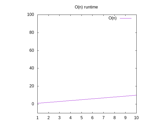
Figure 2: Runtime characteristics of an O(n) function
So what are some other examples of this?
Consider this function:
def is_none(item):
    return item is None
This is a bit of a silly example, but bear with me. This function is
called O(1) which is called "constant time". What this means is no
matter how big our input is, it always takes the same amount of time
to compute things. If you go back to Wolfram and plot 1, you'll see
that it always stays the same, no matter how far right we go. If you
pass in a list of 1 million integers, it'll take about the same time
as if you were going to pass in a list of 1 integer. Constant time is
considered the best case scenario for a function.
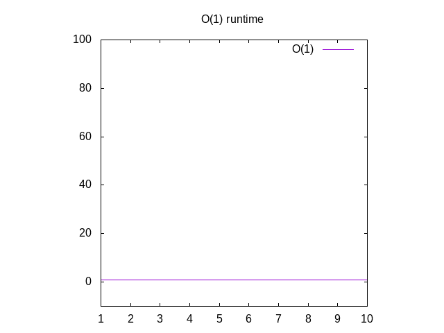
Figure 3: Runtime characteristics of an O(1) function
Consider this function:
def all_combinations(the_list):
   results = []
   for item in the_list:
       for inner_item in the_list:
           results.append((item, inner_item))
   return results
This matches every item in the list with every other item in the
list. If we gave it an array [1,2,3], we'd get back [(1,1) (1,2),
(1,3), (2, 1), (2, 2), (2, 3), (3, 1), (3, 2), (3, 3)]. This is part
of the field of combinatorics (warning: scary math terms!), which is
the mathematical field which studies combinations of things. This
function (or algorithm, if you want to sound fancy) is considered
O(n^2). This is because for every item in the list (aka n for the
input size), we have to do n more operations. So n * n == n^2.
Below is a comparison of each of these graphs, for reference. You can
see that an O(n^2) function will get slow very quickly where as
something that operates in constant time will be much better. This is
particularly useful when it comes to data structures, which I'll post
about soon.
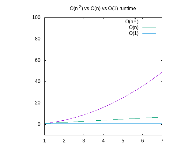
Figure 4: Comparison of O(n2) vs O(n) vs O(1) functions
This is a pretty high level overview of Big-O notation, but hopefully gets you acquainted with the topic. There's a coursera course which can give you a more in depth view into this topic, but be warned that it will hop into mathematic notation very quickly. If anything here doesn't make sense, send me an email.
Update: I've also written about how to calculate Big-O.
I'm thinking of writing a book on this topic. If this is something you'd like to see, please express your interest in it here.
Calculating Big-O
This is the second in a three post series. The first post explains Big-O from a self-taught programmer's perspective. The third article talks about understanding the formal definition of Big-O.
So now that we know what Big-O is, how do we calculate the Big-O classification of a given function? It's just as easy as following along with your code and counting along the way.
  def count_ones(a_list):
      total = 0
      for element in a_list:
          if element == 1:
              total += 1
      return total
The above code is a classic example of an O(n) function. This is
because we have to loop over every element that we get in order to
complete our calculation. We can trace this by following along the
code and counting. We're doing a few calculations here.
- We're setting
totalto zero. - We loop through
a_list. - We check if
elementis equal to 1. - We increment
totalby one a few times.
So setting a counter to zero is a constant time operation. If you
think about what's happening inside the computer, we're setting a
chunk of memory to some new value. Because we've hard-coded the zero
here, it happens in constant time. There's no way to call this
function or alter global state that we could change the
operation. This is an O(1) operation.
Next, we loop through the list. So we have to look at each item in the
list. This number of operations changes depending on the size of the
list. If it's a list of 10 things, we do it 10 times. If it's 75, we do
75 operations. In mathematical terms, this means that the time it
takes to do something increases linearly with its input. We use a
variable to represent the size of the input, which everyone in the
industry calls n. So the "loop over the list" function is O(n)
where n represents the size of a_list.
Checking whether an element is equal to 1 is an O(1) operation. A
way to prove to ourselves that this is true is to think about it as a
function. If we had an is_equal_to_one() function, would it take
longer if you passed in more values (eg is_equal_to_one(4) vs
is_equal_to_one([1,2,3,4,5])? It wouldn't because of the fixed
number 1 in our comparison. It took me a while of conferring with
other people about why this was true before I was convinced. We
decided that binary comparisons are constant time and that's what a
comparison to 1 eventually got to.
Next, we increment total by 1. This is like setting total to zero (but you have to do addition first). Addition of one, like equality, is also constant time.
So where are we? We have \(O(1) + O(n) * (O(1) + O(1))\). This is because we do 1 up front, constant time operation, then (potentially) 2 more constant item things for each item in the list. In math terms, that reduces to \(O(2n) + O(1)\). In big O, we only care about the biggest "term" here. "Term" is the mathematical word that means "portion of an algebraic statement".
To figure out the biggest expression if you don't remember the order,
you can just cheat and graph them. From the other article, we know
that to graph these things you just replace n with x.
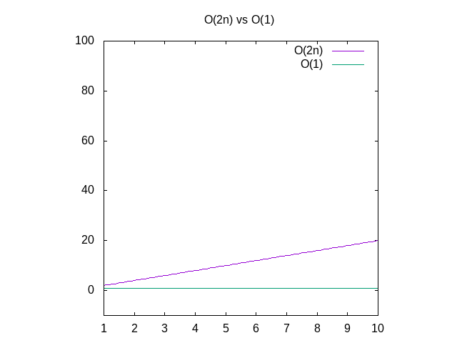
Figure 5: If you don't remember if 2x is bigger than 1, you can always graph them to be sure.
So as I was saying, in calculating Big-O, we're only interested in the
biggest term: O(2n). Because Big-O only deals in approximation, we
drop the 2 entirely, because the difference between 2n and n isn't
fundamentally different. The growth is still linear, it's just a
faster growing linear function. You drop the products of (aka things
multiplying) the variables. This is because these change the rate of
growth, but not the type of growth. If you want a visual indication
of this, compare the graph of x^2 vs 2x vs x. x^2 is a
different type of growth from the other two (quadratic [which is
just a math-y way of saying "squared"] vs linear), just like 2n is a
different type of growth from 1 in the graph above (linear vs
constant). Even if you pick a really high multiplier like 10,000, we
can still beat it with x^2 because eventually the line for x^2 will
be higher if we go far enough to the right.
To sum it up, the answer is this function has an O(N) runtime (or a
linear runtime). It runs slower the more things you give it, but that
should grow at a predictable rate.
The key aspects to determining the Big-O of a function is really just as simple as counting. Enumerate the different operations your code does (be careful to understand what happens when you call out into another function!), then determine how they relate to your inputs. From there, its just simplifying to the biggest term and dropping the multipliers.
If you found this interesting, I'm thinking about writing up a longer form book on this topic. Head over to leanpub and express your interest in hearing more. If you have any questions, please feel free to email me.
Thanks to Wraithan, Chris Dickinson and Cory Kolbeck for their review.